Computer Graphics: A Shortcut
Most introductions to computer graphics begin with triangular meshes and a graphics API — a steep entry cost even for legacy APIs like OpenGL, and steeper still for modern ones. This demo is intended for those with no prior graphics experience who want to understand 3D surface rendering without that overhead. We illustrate the core principles through direct manipulation of real geospatial data.
Most graphics courses build rendering on top of triangular meshes, but the lighting model itself requires only a surface normal. A digital elevation model (DEM) supplies normals directly, bypassing mesh construction entirely. As a single-valued height function $f(x,y)$, a DEM also has no backfaces — every surface point faces upward and is always visible from above, eliminating visibility and occlusion checks. This reduces 3D surface rendering to an image filter: iteration over pixels, a local stencil to approximate the surface normal from neighboring height values, and basic arithmetic for the lighting equation.
We implement Phong shading from scratch in Python over a real LiDAR DEM (Illinois statewide survey). An interactive widget exposes the shading parameters — light direction, ambient, diffuse, specular coefficients — so the reader can feel the effect of each before its formula is introduced.
import matplotlib.pyplot as plt

dem = plt.imread('IL_Statewide_Lidar_DEM_WGS.png')[:,:,0]
plt.imshow(dem, cmap='gray', vmin=0, vmax=1)
<matplotlib.image.AxesImage at 0x1292e87d0>

Geometry Fundamentals
3D Vector
$\vec{u} = (\Delta x, \Delta y, \Delta z)$, 3 components.
Dot product
Dot product of two vectors $\operatorname{dot}(\vec{a}, \vec{b})$ measure the "closeness" of the two vectors.
Imagine: n = feet--torso-->head and l = shoulder--arm-->hand ... sun. Dot products translates to soreness in your shoulder.
- noon: $\operatorname{dot}(\vec{n}, \vec{l})\approx 1$
- morning/afternoon: $0 < \operatorname{dot}(\vec{n}, \vec{l}) < 1$
- dawn/dusk: $\operatorname{dot}(\vec{n}, \vec{l}) \approx 0$
- night: $\operatorname{dot}(\vec{n}, \vec{l}) < 0$
All surfaces are similar to the Earth's surface. (GEOmetry!) The local days and nights serve as a visual cue for our 3D perception.
We need two things: a light direction $\vec{l}$ and a surface normal $\vec{n}$. We also need to normalize them first.
import numpy as np
from numba import njit, prange

@njit
def normalize(v):
    return v / np.linalg.norm(v)
Light Direction
We use two angles $\theta$ and $\psi$ to describe the light direction:
$$\vec{l}(\theta, \psi) = \left(\cos\theta\cos\psi, \cos\theta\sin\psi, \sin\theta \right)$$

@njit
def light(theta, psi):
    l = np.array([
        np.cos(np.radians(theta)) * np.cos(np.radians(psi)),
        np.cos(np.radians(theta)) * np.sin(np.radians(psi)),
        np.sin(np.radians(theta))
    ])
    return normalize(l)
Surface Normal
Cross product
$\operatorname{cross}(\vec{a}, \vec{b}) = \vec{a} \times \vec{b}$ is perpendicular to both $\vec{u}$ and $\vec{v}$.

Example: DEM
Let's focus on a hypothetical example around point $(i, j)$
                (i-1, j)
(i-1, j-1) ?--------4--------? (i-1, j+1)
           |        ^        |
           |        ^        |
  (i, j-1) 3>>>>>>(i,j)>>>>>>2 (i, j+1)
           |        ^        |
           |        ^        |
(i+1, j-1) ?--------1--------? (i+1, j+1)
                (i+1,j)
$$\vec{t}_x = (2, 0, dem[i, j+1] - dem[i, j-1]) = (2, 0, 2-3) = (2, 0, -1)$$ $$\vec{t}_y = (0, 2, dem[i-1, j] - dem[i+1, j]) = (0, 2, 4-1) = (0, 2, 3)$$ $$\vec{n} = \operatorname{cross}(\vec{t}_x, \vec{t}_y) = \operatorname{cross}((2, 0, -1), (0, 2, 3)) = (2, -6, 4)$$
For the mathematically-inclined
A function $f(x,y)$ defines a surface $$\vec{r}(x, y) = (x, y, f(x, y))^\top.$$ The tangent vectors are: $$\frac{\partial \vec{r}}{\partial x}(x,y) = \left(1, 0, \frac{\partial f}{\partial x}(x, y)\right)^\top, \quad \frac{\partial \vec{r}}{\partial y}(x,y) = \left(0, 1, \frac{\partial f}{\partial x}(x, y)\right)^\top.$$ The (unnormalized) normal vector is the cross product of the two: $$\vec{n}(x,y) = \frac{\partial \vec{r}}{\partial x}(x,y) \times \frac{\partial \vec{r}}{\partial y}(x,y) = \left(-\frac{\partial f}{\partial x}(x, y), -\frac{\partial f}{\partial y}(x, y), 2\right)^\top.$$ The first order approximation (i.e. finite difference) of the normal is: $$\vec{n}[i,j] = \left(\frac{f[i, j-1] - f[i, j+1]}{2h}, \frac{f[i+1,j] - f[i-1,j]}{2h}, 2\right)^\top.$$@njit
def normal(dem, i, j):
"""
This will be stubbed out
"""
tx = np.array([2., 0., dem[i, j + 1] - dem[i, j - 1]])
ty = np.array([0., 2., dem[i - 1, j] - dem[i + 1, j]])
n = np.cross(tx, ty)
return normalize(n)
Computer Graphics Primer
Phong Shading (1975)
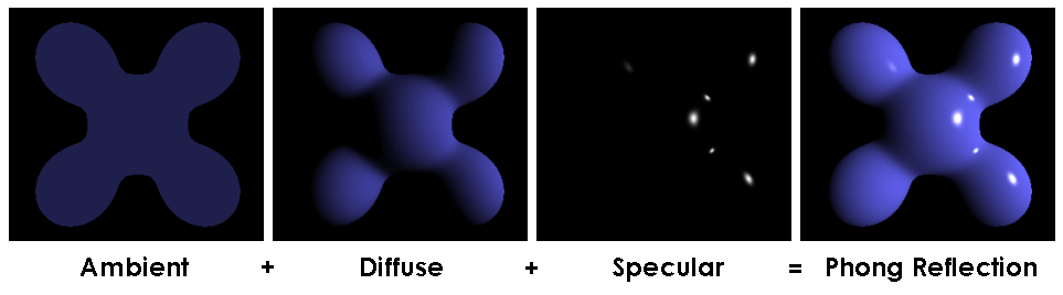
Given surface normal (unit vector) $\vec{n}$, light direction (unit vector) $\vec{l}$, and eye direction (unit vector) $\vec{v}$, we can break down pixel's color intensity into three components:
- ambient lighting: $k_{a} \cdot \vec{I}_a \odot \vec{C}$
- diffuse lighting: $k_{d} \cdot \operatorname{dot}(\vec{l}, \vec{n}) \cdot \vec{I} \odot \vec{C}$
- specular lighting: $k_{s} \cdot \operatorname{dot}(\vec{r}, \vec{v})^r \cdot \vec{I} \odot \vec{C}$. where the reflected light direction (unit vector) is: $$\vec{r} = 2 \cdot \operatorname{dot}(\vec{l},\vec{n}) \cdot \vec{n} - \vec{l}$$
($\cdot$ means scalar multiplication, i.e. *. $\odot$ means element-wise multiplication, i.e. * or np.multiply.)
@njit
def color(dem, i, j):
    t = dem[i, j]
    c1 = np.array([0.5, 0.2, 0.2])
    c2 = np.array([1., 1., 1.])
    return (1 - t) * c1 + t * c2
    # return np.ones(3)
@njit(parallel=True)
def render(dem, exaggeration, theta, psi, k_a, k_d, k_s, gamma):
    exaggerated = dem * exaggeration

    # Play with this
    lights = [
        (light(theta, psi), np.array([1., 0.5, 0.])),
        (light(theta, psi + 100.), np.array([0., 0.5, 1.])),
        (light(theta, psi + 200.), np.array([0.5, 0.5, 0.5]))
        # (light(theta, psi), np.ones(3))
    ]

    # We are looking at the terrain from above
    v = np.array([0., 0., 1.])

    def shade_pixel(i, j):
        """
        This function will be stubbed out
        """
        C = color(dem, i, j)
        n = normal(exaggerated, i, j)

        pixel = np.zeros(3)

        for l, I in lights:
            ambient = k_a * I * C

            d = l.dot(n)
            diffuse = k_d * d * I * C

            r = n * 2 * d - l
            specular = k_s * r.dot(v) ** gamma * I * C

            pixel += ambient + diffuse + specular

        return pixel

    H, W = dem.shape
    out = np.zeros((H, W, 3))
    for i in prange(1, H - 1):
        for j in prange(1, W - 1):
            out[i, j] = shade_pixel(i, j)

    return out.clip(0, 1)
from timeit import default_timer as timer
from ipywidgets import interact, interactive

def draw(exaggeration=30, theta=20, psi=0, k_a=0., k_d=0.5, k_s=0.5, gamma=6):
    start = timer()
    out = render(dem, exaggeration, theta, psi, k_a, k_d, k_s, gamma)
    end = timer()
    print(f'Render time: {end - start}s', end='\r')
    plt.figure('naive', figsize=(8,8))
    plt.imshow(out)

draw()
Render time: 1.6411467919970164s

widget = interactive(draw, exaggeration=(0,50), theta=(0,90), psi=(0,360), k_a=(0,1.), k_d=(0,1.), k_s=(0,1.), gamma=(1,10))
widget.children[-1].layout.height = '8in'
widget
interactive(children=(IntSlider(value=30, description='exaggeration', max=50), IntSlider(value=20, description…